HTTP Requests
HTTP stands for Hyper Text Transfer Protocol. This protocol (like many) was proposed by the Internet Engineering Task Force (IETF) through a request for comments (RFC). We're going to start with a very simple HTTP method: the get method.
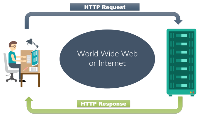
To learn more about HTTP methods see:
https://developer.mozilla.org/en-US/docs/Web/HTTP/Methods
Python's Requests Package
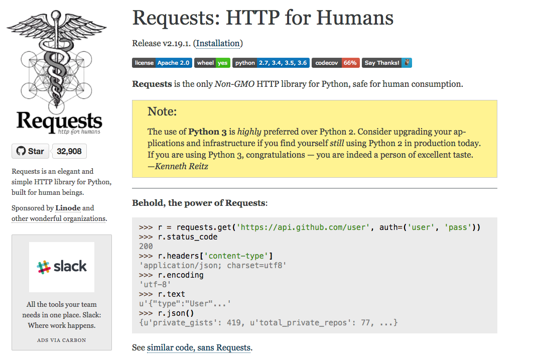
The first thing to understand when dealing with APIs is how to make get requests in general. To do this, we'll use the Python requests package.
http://docs.python-requests.org/en/master/
import requests
response = requests.get('https://flatironschool.com')
print('Type:', type(response), '\n')
print('Response:', response, '\n')
print('Response text:\n', response.text)
Hmmm, well that was only partially helpful. You can see that our request was denied. (This is shown by the response itself, which has the code 403, meaning forbidden.) Most likely, this is caused by permissioning from Flatiron School's servers, which may be blocking requests that appear to be from an automated platform.
HTTP Response Codes
In general, here's some common HTTP response codes you might come across:

Let's try another get request in the hopes of getting a successful (200) response.
#The Electronic Frontier Foundation (EFF) website; advocating for data privacy and an open internet
response = requests.get('https://www.eff.org')
print(response)
print(response.text[:2500])
Success! As you can see, the response.text is the html code for the given url that we requested. In the background, this forms the basis for web browsers themselves. Every time you put in a new url or click on a link your computer makes a get request for that particular page and then the browser itself renders that page into a visual display on screen.
OAuth
Some requests are a bit more complicated. Often, websites require identity verification such as logins. This helps a variety of issues such as privacy concerns, limiting access to content and tracking users history. Going forward, OAuth has furthered this idea by allowing third parties such as apps access to user information without providing the underlying password itself.
In the words of the Internet Engineering Task Force, "The OAuth 2.0 authorization framework enables a third-party application to obtain limited access to an HTTP service, either on behalf of a resource owner by orchestrating an approval interaction between the resource owner and the HTTP service, or by allowing the third-party application to obtain access on its own behalf. This specification replaces and obsoletes the OAuth 1.0 protocol described in RFC 5849."
See https://oauth.net/2/ or https://tools.ietf.org/html/rfc6749 for more details.
Access Tokens
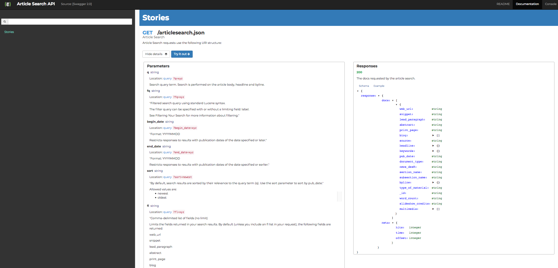
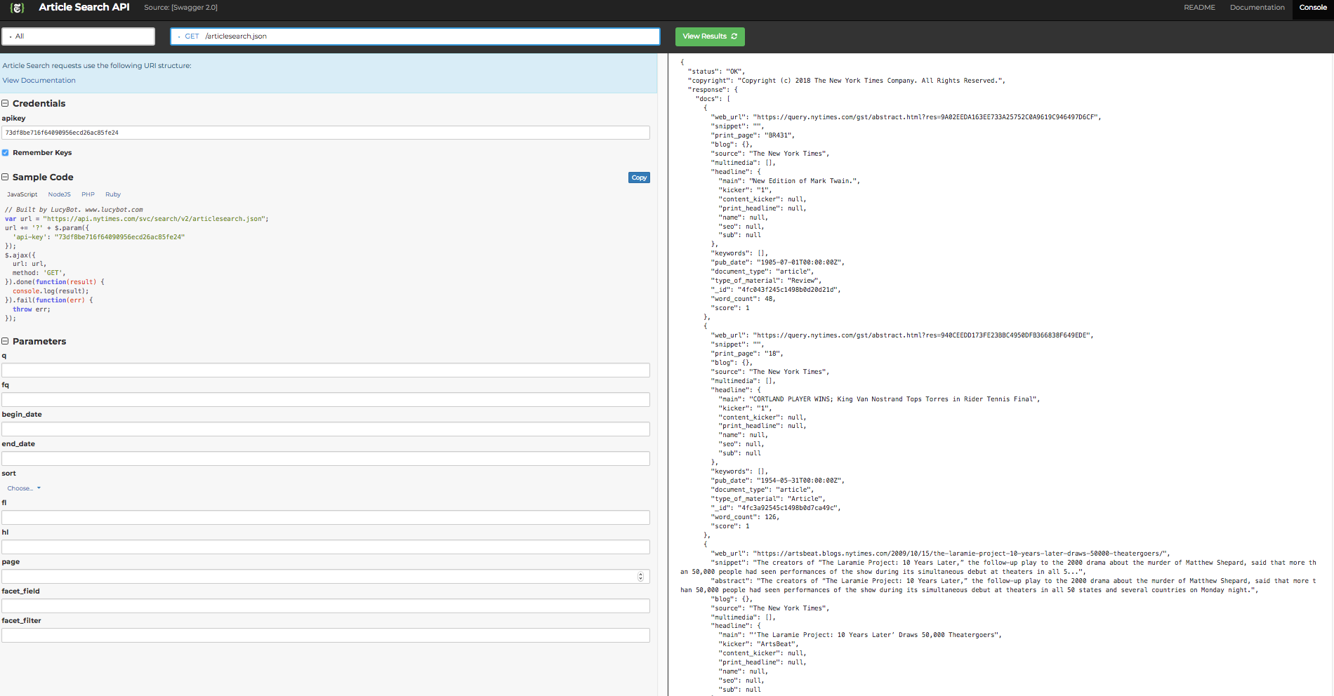
In order to make requests to many APIs, you are required to login via an access token. As a result, the first step is to sign up through the web interface using your browser. Once you have an API key, you can then use it to make requests to the API. As with login passwords for your computer, these access tokens should be kept secret! For example, rather then including the passwords directly in this file, I have saved them to a seperate file called 'ny_times_api_keys.py'. The file would look something like this:
api_key = 'blah_blah_blah_YOUR_KEY_HERE'
Now it's time to start making some api calls!
from ny_times_api_keys import *
import requests
url = "https://api.nytimes.com/svc/search/v2/articlesearch.json"
url_params = {"api-key" : api_key,
             'fq' : 'The New York Times',
             'sort' : "newest"}
response = requests.get(url, params=url_params)
response
JSON Files
While you can see that we received an HTTP code of 200, indicating success, the actual data from the request is stored in a json file format. JSON stands for Javascript Object Notation and is the standard format for most data requests from the web these days. You can read more about json here. With that, let's take a quick look at our data:
response.json()
type(response.json())
response.json()['response']['docs'][0]['web_url']
response.json()['response']['docs'][0]['headline']
import pandas as pd
pd.DataFrame(response.json()['response']['docs'])
import time
responses = []
for i in range(10**3):
    url = "https://api.nytimes.com/svc/search/v2/articlesearch.json"
    url_params = {"api-key" : api_key,
                 'fq' : 'The New York Times',
                  'q' : 'politics',
                  'sort' : "newest",
                 'page': i}
    response = requests.get(url, params=url_params)
    if response.status_code == 200:
        responses.append(response)
    else:
        print('Request Failed.')
        print(response)
        print('Pausing for 60 seconds.')
        time.sleep(60)
    time.sleep(2) #Always include a 2 second pause
print(len(responses))
dfs = []
for r in responses:
    dfs.append(pd.DataFrame(r.json()['response']['docs']))
df = pd.concat(dfs, ignore_index=True)
print(len(df))
df.head()
df['main_headline'] = df.headline.map(lambda x: x['main'])
text = ''
for h in df.main_headline:
    text += str(h)
print(len(text), text[:50], text[-50:])
df.to_csv('Pulls_Nov1_2018_recent.csv', index=False)
import pandas as pd
df = pd.read_csv('Pulls_Nov1_2018_recent.csv')
df.head()
import matplotlib.pyplot as plt
import seaborn as sns
# sns.set_style('darkgrid')
%matplotlib inline
df.word_count.hist(figsize=(10,10))
plt.title('Distribution of Words Per Article')
plt.xlabel('Number of Words in Articles')
plt.ylabel('Number of Articles')
word_counts = {}
for h in df.main_headline:
    for word in h.split():
        word = word.lower()
        word_counts[word] = word_counts.get(word, 0) + 1
word_counts = pd.DataFrame.from_dict(word_counts, orient='index')
word_counts.columns = ['count']
word_counts = word_counts.sort_values(by='count', ascending=False)
word_counts.head(10)
word_counts.head(25).plot(kind='barh', figsize=(12,10))
plt.title('Most Frequent Headline Words',  fontsize=18)
plt.xlabel('Frequency', fontsize=14)
plt.ylabel('Word',  fontsize=14)
plt.xticks( fontsize=14)
plt.yticks( fontsize=14)
Topic Modelling
Brief Background
In order to perform topic modelling on our data we will use two primary tools. The first is to turn our text into a vector of word frequency counts; each possible word will be a feature and the number of times that word occurs will be represented by a number. From there, we can then apply mathematical operations to this numerical representation. In our case, we will be applying a common Natural Language Processing Algorithm known as Latent Dirichlet Allocation (LDA). For more technical details, start here.
from sklearn.feature_extraction.text import CountVectorizer
corpus = [
        'This is the first document.',
        'This document is the second document.',
        'And this is the third one.',
        'Is this the first document?',
        ]
vectorizer = CountVectorizer()
X = vectorizer.fit_transform(corpus)
print(vectorizer.get_feature_names())
print(X.toarray())
#Installing a new python package on the fly
!pip install lda
LDA: Latent Dirichlet Allocation
https://en.wikipedia.org/wiki/Latent_Dirichlet_allocation
http://jmlr.org/papers/volume3/blei03a/blei03a.pdf
Latent dirichlet allocation is a probabilistic model for classifying documents. It works by viewing documents as mixtures of topics. In turn, topics can be viewed of as probability distributions of words. As we'll see, this allows us to model topics of a corpus and then visualize these topics by the top words associated with the topics as word clouds. While the mathematics behind LDA is fairly complex and outside the scope of this presentation, you can easily implement this powerful concept using prebuilt tools based on this academic research.
from sklearn.feature_extraction.text import CountVectorizer
import lda
import numpy as np

tf_vectorizer = CountVectorizer(max_df=0.95, min_df=2, max_features=10000,
                                stop_words='english');
tf = tf_vectorizer.fit_transform(df.main_headline);


model = lda.LDA(n_topics=6, n_iter=1500, random_state=1);
model.fit(tf);

topic_word = model.topic_word_  # model.components_ also works
vocab = tf_vectorizer.get_feature_names();
n_top_words = 10
for i, topic_dist in enumerate(topic_word):
    topic_words = np.array(vocab)[np.argsort(topic_dist)][:-(n_top_words):-1]
    print('Topic {}: {}'.format(i, ' '.join(topic_words)))
from wordcloud import WordCloud

topic = "new soviet russia national talks party music world minister"
# Generate a word cloud image
wordcloud = WordCloud().generate(topic)

# Display the generated image:
# the matplotlib way:
import matplotlib.pyplot as plt
plt.imshow(wordcloud, interpolation='bilinear')
plt.axis("off")

# lower max_font_size
wordcloud = WordCloud(max_font_size=40).generate(topic)
plt.figure()
plt.imshow(wordcloud, interpolation="bilinear")
plt.axis("off")
plt.show()
sns.set_style(None)
fig, axes = plt.subplots(3,2, figsize=(15,15))
fig.tight_layout()
for i, topic_dist in enumerate(topic_word):
    topic_words = list(np.array(vocab)[np.argsort(topic_dist)][:-(n_top_words):-1])
    topic_words = ' '.join(topic_words)
    row = i//2
    col = i%2
    ax = axes[row, col]
    wordcloud = WordCloud().generate(topic_words)
    ax.imshow(wordcloud, interpolation='bilinear')
    ax.set_title('Topic {}'.format(i))
plt.tight_layout()
Summary
Congratulations! We've covered a lot here! We started with HTTP requests, one of the fundamental protocols underlying the internet that we know and love. From there, we further investigated OAuth and saw how to get an access token to use in an API such as yelp. Then we made some requests to retrieve information that came back as a json format. We then transformed this data into a dataframe using the Pandas package. Finally, we created an initial visualization of the data that we retrieved using matplotlib!
from bs4 import BeautifulSoup
def scrape_full_article_text(url):
    response = requests.get(url)
    page = response.text
    soup = BeautifulSoup(page, 'html.parser')
    paragraphs = soup.find_all('p', attrs={'class': 'story-body-text'})
    full_text=str()
    for paragraph in paragraphs:
        raw_paragraph = paragraph.contents
        cleaned_paragraph=str()
        for piece in raw_paragraph:
            if piece.string:
                cleaned_paragraph += piece.string
                cleaned_paragraph = cleaned_paragraph.replace(r"<.*?>","")
                cleaned_paragraph = cleaned_paragraph.encode('ascii','ignore')
                print(cleaned_paragraph, type(cleaned_paragraph))
        full_text += str(cleaned_paragraph)
    return full_text

